04 - Modern CNNs

References

• Reading: Dive into Deep Learning (D2L), Modern Convolutional Neural Networks

在 LeNet 之后, CNN 并没有立即流行起来. 计算效率的不足以及许多神经网络的训练技巧 (如 parameter initialization, effective regularization 等) 的缺乏, 使得 CNN 的训练变得非常困难.

直到 2012 年, AlexNet 在 ImageNet 竞赛中取得了巨大的成功, CNN 才开始流行起来. 这也标志着深度学习的新时代. 一个主流的想法是: 通过增加网络的深度, 使得浅层的网络学习局部的特征(如边缘, 颜色, 纹理等)而深层的网络学习全局的特征(如物体, 形状等). 这使得 CNN 在图像分类, 目标检测, 图像分割等任务中取得了巨大的成功. 虽然深度神经网络的概念非常简单, 但由于不同的网络架构和超参数选择, 这些神经网络的性能会发生很大变化.

这些模型包括：

• AlexNet: 它是第一个在大规模视觉竞赛中击败传统计算机视觉模型的大型神经网络；
• VGG-Net: 它利用许多重复的神经网络块；
• Network in Network (NiN): 它重复使用卷积层和卷积层（用来代替全连接层）来构建深层网络；
• GoogLeNet: 它使用并行连结的网络，通过不同窗口大小的卷积层和最大汇聚层来并行抽取信息；
• ResNet: 它使用残差块来构建跨层的数据通道，是计算机视觉中最流行的体系架构；
• DenseNet: 它的计算成本很高，但给我们带来了更好的效果。

这些模型是按照时间顺序排列的. 这些模型是将人类直觉和相关数学见解结合后, 经过大量研究试错后的结晶.

1. Missing Ingredients Before AlexNet

在 AlexNet 之前, 深层神经网络的训练非常困难. 主要是由于以下几个原因:

DATA

• 深层的神经网络需要大量的数据来进行训练. 但在之前, 研究者们并没有足够的数据 (以及足够的存储能力) 来训练深层的神经网络.
• 在 2009 年发布了 ImageNet 数据集, 该数据集包含了 $1000000$ 张图像 ($1000$ 类别, 每个类别 $1000$ 张图像), 并且图像的分辨率高达 $224\times 224$.
• 相应的, ImageNet Large Scale Visual Recognition Challenge (ILSVRC) 竞赛也开始举办, 促进了计算机视觉领域的研究.

HARDWARE

• GPU 由于其并行计算的能力, 使得深层神经网络的训练变得可行.
• 在 2004 年, NVIDIA 开始在 GPU 上优化通用计算的能力.
• CPU 的每个核心都拥有高频率运行的能力, 其非常适合运行各种指令, 但它们在任何单个任务上的性能都相对较差
• 而 GPU 由 $100\sim 1000$ 个小的处理单元组成, 尽管每个小的处理单元的性能较差, 但是庞大的数量使得 GPU 在并行计算上非常强大.
• 在 2012 年, Alex Krizhevsky 等人意识到了深度神经网络中的瓶颈矩阵乘法可以被 GPU 的并行计算所加速, 成功地使用两个显存为3GB的NVIDIA GTX580 GPU 实现了快速卷积运算, 推动了深度学习的研究.

2. AlexNet

AlexNet 是第一个在大规模视觉竞赛中击败传统计算机视觉模型的大型神经网络 (即一个学习到的网络的效果优于了传统人为设计的网络), 由 Alex Krizhevsky, Ilya Sutskever 和 Geoffrey Hinton 在 2012 年提出. 它在 ImageNet 竞赛中取得了巨大的成功.

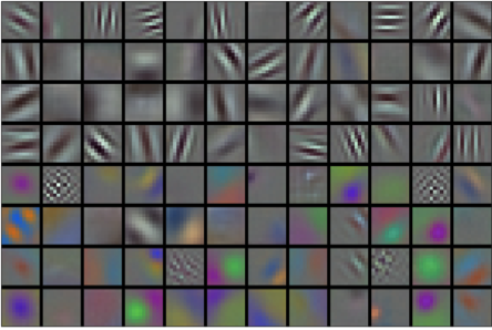
其中, AlexNet 的网络结构如下:

• 可以发现, AlexNet 的网络结构比 LeNet 更深, 其包含了 $5$ 个卷积层, 并且每个卷积层的 Kernel 大小也都更大
• AlexNet 使用了 ReLU 激活函数 (而不是 sigmoid)
  • ReLU 的计算速度更快 (不需要计算指数函数)
  • 在训练过程中, ReLU 的梯度不会消失 (sigmoid 的梯度在 $x$ 取值较大或较小时会趋近于 $0$)
• AlexNet 从 Average Pooling 改为 Max Pooling
• AlexNet 使用了 Dropout 来防止过拟合, 而 LeNet 只使用了 weight decay

其 Python 实现如下:

import torch
import torch.nn as nn
 
class AlexNet(nn.Module):
    def __init__(self, num_classes=1000):
        super(AlexNet, self).__init__()
        self.features = nn.Sequential(
            # Layer 1
            nn.Conv2d(3, 96, kernel_size=11, stride=4, padding=2),  # Input: 224x224x3, Output: 55x55x96
            nn.ReLU(inplace=True),
            nn.MaxPool2d(kernel_size=3, stride=2),  # Output: 27x27x96
 
            # Layer 2
            nn.Conv2d(96, 256, kernel_size=5, padding=2),  # Output: 27x27x256
            nn.ReLU(inplace=True),
            nn.MaxPool2d(kernel_size=3, stride=2),  # Output: 13x13x256
 
            # Layer 3
            nn.Conv2d(256, 384, kernel_size=3, padding=1),  # Output: 13x13x384
            nn.ReLU(inplace=True),
 
            # Layer 4
            nn.Conv2d(384, 384, kernel_size=3, padding=1),  # Output: 13x13x384
            nn.ReLU(inplace=True),
 
            # Layer 5
            nn.Conv2d(384, 256, kernel_size=3, padding=1),  # Output: 13x13x256
            nn.ReLU(inplace=True),
            nn.MaxPool2d(kernel_size=3, stride=2),  # Output: 6x6x256
        )
 
        self.classifier = nn.Sequential(
            # Fully connected layers
            nn.Dropout(0.5),
            nn.Linear(256 * 6 * 6, 4096),
            nn.ReLU(inplace=True),
 
            nn.Dropout(0.5),
            nn.Linear(4096, 4096),
            nn.ReLU(inplace=True),
 
            nn.Linear(4096, num_classes),
        )
 
    def forward(self, x):
        x = self.features(x)
        x = torch.flatten(x, 1)  # Flatten the feature maps
        x = self.classifier(x)
        return x
 
# Example usage
if __name__ == '__main__':
    # Create an instance of AlexNet
    model = AlexNet()
 
    # Create a random input tensor (batch_size, channels, height, width)
    # AlexNet expects 224x224 RGB images
    sample_input = torch.randn(1, 3, 224, 224)
 
    # Forward pass
    output = model(sample_input)
 
    print(f"Model output shape: {output.shape}")
    print(model)

3. VGG-Net

不论是 LeNet 还是 AlexNet, 其核心的思想都是用一些 CNN 层来提取特征, 然后用一些全连接层来进行分类, 中间可能会有一些 pooling 层来进行下采样. 然而随着网络的加深, spatial resolution 会迅速减小, 这使得网络的深度受到限制.

• 例如对于一个 $d\times d$ 的图像, 如果使用 $2\times 2$ 的 pooling 层, 那么每次下采样都会将图像的大小减半, 因此最多只能进行 $\mathcal{O}({\log }_{2}d)$ 次下采样. 而这也给出了模型的深度的上限.
• 然而模型的深度是影响模型性能的一个重要因素.
  • 例如对于一个 $5\times 5$ 的 receptive field, 我们既可以使用一个 $5\times 5$ 的 kernel 来提取特征, 也可以使用 $2$ 层 $3\times 3$ 的 kernel 来提取特征. 然而实验表明, 使用 $2$ 层 $3\times 3$ 的 kernel 来提取特征的效果要比使用一个 $5\times 5$ 的 kernel 来提取特征的效果要好.
  • Narrow & Deep 要比 Shallow & Wide 的效果要好.

随着 Transfer Learning 的发展, 研究者们逐渐转为以 Layers 和 Blocks 为单位来设计网络, 并且从一个大规模 pre-trained 的网络中迁移到不同的任务上. 在 CNN 领域, 研究者提出了以 Blocks 为单位的 Multiple Convolutional Layers 的设计.

VGG-Net 就是一个由 Blocks 组成的网络, 由 Visual Geometry Group 在 2014 年提出. VGG-Net 的网络结构如下:

VGG-Net 包含两个大的模块: Convolutional+Pooling 和 Fully Connected

• Fully Connected 模块的设计与 AlexNet 完全相同
• Convolutional+Pooling 模块的设计与 AlexNet 有所不同, 其设计的架构是以 Blocks 为单位的. 一个 Block 由若干 $3\times 3$ 的卷积层 (padding=1) 和最后一个 $2\times 2$ 的 pooling 层 (stride=2) 组成.
  • 对于一个 $3\times 3$, padding=1 的卷积层, 其输出的 spatial resolution 和输入的 spatial resolution 是相同的 ($n+2\times 1-3+1=n$).
  • 对于一个 $2\times 2$, stride=2 的 pooling 层, 其输出的长度和宽度都是输入的一半 ($\frac{n}{2}$).

一个 VGG-Block 的设计如下:

def vgg_block(in_channels, out_channels, num_convs):
    """
    Basic VGG block
    Args:
        in_channels: Number of input channels
        out_channels: Number of output channels
        num_convs: Number of convolutional layers in the block
    Returns:
        A sequential module containing the VGG block
    """
    layers = []
 
    # First convolutional layer (input channels -> output channels)
    layers.append(nn.Conv2d(in_channels, out_channels, kernel_size=3, padding=1))
    layers.append(nn.ReLU(inplace=True))
 
    # Additional convolutional layers (output channels -> output channels)
    for _ in range(num_convs - 1):
        layers.append(nn.Conv2d(out_channels, out_channels, kernel_size=3, padding=1))
        layers.append(nn.ReLU(inplace=True))
 
    # Max pooling at the end of the block
    layers.append(nn.MaxPool2d(kernel_size=2, stride=2))
 
    return nn.Sequential(*layers)

当我们定义了一个 VGG-Block 之后, 我们就可以使用它来构建 VGG-Net 了. 一个典型例子 VGG-11 的网络结构如下:

class VGG11(nn.Module):
    def __init__(self, num_classes=1000):
        super(VGG11, self).__init__()
 
        # VGG-11 configuration: 1-1-2-2-2 convolutional layers per block
        # First block: 1 conv layer with 64 filters
        self.block1 = vgg_block(3, 64, 1)
 
        # Second block: 1 conv layer with 128 filters
        self.block2 = vgg_block(64, 128, 1)
 
        # Third block: 2 conv layers with 256 filters
        self.block3 = vgg_block(128, 256, 2)
 
        # Fourth block: 2 conv layers with 512 filters
        self.block4 = vgg_block(256, 512, 2)
 
        # Fifth block: 2 conv layers with 512 filters
        self.block5 = vgg_block(512, 512, 2)
 
        # Classifier part (fully connected layers)
        self.classifier = nn.Sequential(
            nn.Flatten(),
            nn.Linear(512 * 7 * 7, 4096),
            nn.ReLU(True),
            nn.Dropout(p=0.5),
            nn.Linear(4096, 4096),
            nn.ReLU(True),
            nn.Dropout(p=0.5),
            nn.Linear(4096, num_classes)
        )
 
        # Initialize weights
        self._initialize_weights()
 
    def forward(self, x):
        # Pass input through each block
        x = self.block1(x)
        x = self.block2(x)
        x = self.block3(x)
        x = self.block4(x)
        x = self.block5(x)
 
        # Pass through classifier
        x = self.classifier(x)
        return x
 
    def _initialize_weights(self):
        for m in self.modules():
            if isinstance(m, nn.Conv2d):
                nn.init.kaiming_normal_(m.weight, mode='fan_out', nonlinearity='relu')
                if m.bias is not None:
                    nn.init.constant_(m.bias, 0)
            elif isinstance(m, nn.Linear):
                nn.init.normal_(m.weight, 0, 0.01)
                nn.init.constant_(m.bias, 0)
 
# Example usage
if __name__ == '__main__':
    # Create a VGG-11 model
    model = VGG11()
 
    # Create a sample input tensor (batch_size=1, channels=3, height=224, width=224)
    x = torch.randn(1, 3, 224, 224)
 
    # Forward pass
    output = model(x)
 
    # Print model architecture
    print(model)
 
    # Print output shape
    print(f"Output shape: {output.shape}")

• 在最原始的 VGG 中一共包含了 $5$ 个 VGG-Block, 其中前两个 Block 中只有 $1$ 个卷积层, 后面三个 Block 中有 $2$ 个卷积层 (因此一共有 $2\times 1+3\times 2=8$ 个卷积层 + $3$ 个全连接层), 故也称为 VGG-11.
• 第一个 Block 的输入通道数为 $3$, 输出通道数为 $64$; 第二个 Block 的输出通道数为 $128$; 第三个为 $256$; 第四个为 $512$; 第五个为 $512$.
• _initialize_weights 函数用于初始化网络的权重. 其会遍历网络中的每一层, 如果是卷积层, 则使用 Kaiming Normal 初始化权重, 如果是全连接层, 则使用均值为 $0$, 方差为 $0.01$ 的正态分布初始化权重.
• VGG-Net 的参数量非常大, 其在 ImageNet 上的参数量为 $138$M, 而 AlexNet 的参数量为 $60$M.

4. Network in Network (NiN)

不论是 LeNet, AlexNet 还是 VGG-Net, 其整体的架构都是前面用卷积层提取特征, 后面用全连接层进行分类. 但是这里有两个主要问题:

• 随着网络的加深, 全连接层的参数量会迅速增大, 这使得网络的训练变得非常困难.
• 并且这个线性层只能在最后一层使用 (否则会破坏卷积层的空间结构), 这使得网络的表达能力受到限制.

Network in Network (NiN) (2013) 则提出了一个新的思路:

• 引入了 $1\times 1$ 的卷积层, 这样就可以在卷积层中使用非线性激活函数, 使得网络的表达能力更强.
• 在最后一层引入 Global Average Pooling (GAP), 整合了卷积层的整体空间结构, 使得网络的参数量大大减少.

NiN 的网络结构如下:

• NiN 借鉴了 VGG 的 Block 的设计以及 AlexNet 的参数设置. 具体而言, NiN 中一共有 $4$ 个 Block, 每个 Block 中有 $1$ 个正常的卷积层和 $2$ 个 $1\times 1$ 的卷积层. 并且这四个 Block 中的正常卷积层的参数分别为: 11*11, channels=96, stride=4 → 5*5, channels=256, padding=2 → 3*3, channels=384, padding=1 → 3*3, channels=10, padding=1.
• 注意到, 在 NiN 中, 最后一个 Block 的输出通道数恰好为要分类的类别数 (以替换掉全连接层).
• 紧接着对于最后一个 Block 的输出, 由于其有 num_classes 个通道, 我们对每个通道都各自进行一次 Global Average Pooling, 也就是对每个通道的 $h\times w$ 的特征图求一个平均值. 因此我们会得到 num_classes 个 $1\times 1$ 的特征图 (即每个通道的平均值). 最后我们就可以直接利用这个平均值来进行分类了.

NiN 的 Block 的设计如下:

def nin_block(in_channels, out_channels, kernel_size, stride, padding):
    """
    Network in Network (NiN) block
    """
    return nn.Sequential(
        # Regular convolution layer
        nn.Conv2d(in_channels, out_channels, kernel_size, stride, padding),
        nn.ReLU(inplace=True),
        # 1x1 convolution (mlpconv) for feature combination
        nn.Conv2d(out_channels, out_channels, kernel_size=1),
        nn.ReLU(inplace=True),
        # Another 1x1 convolution (mlpconv) for feature combination
        nn.Conv2d(out_channels, out_channels, kernel_size=1),
        nn.ReLU(inplace=True)
    )

在定义了 NiN 的 Block 之后, 我们就可以使用它来构建 NiN:

class NiN(nn.Module):
    def __init__(self, num_classes=1000):
        super(NiN, self).__init__()
 
        self.features = nn.Sequential(
            # First NiN block
            nin_block(3, 96, kernel_size=11, stride=4, padding=0),
            nn.MaxPool2d(kernel_size=3, stride=2),
            nn.Dropout(0.2),
 
            # Second NiN block
            nin_block(96, 256, kernel_size=5, stride=1, padding=2),
            nn.MaxPool2d(kernel_size=3, stride=2),
            nn.Dropout(0.2),
 
            # Third NiN block
            nin_block(256, 384, kernel_size=3, stride=1, padding=1),
            nn.MaxPool2d(kernel_size=3, stride=2),
            nn.Dropout(0.2),
 
            # Fourth NiN block - replaces fully connected layers
            nin_block(384, num_classes, kernel_size=3, stride=1, padding=1),
 
            # Global average pooling to generate the final output
            nn.AdaptiveAvgPool2d((1, 1))
        )
 
        # Initialize weights
        self._initialize_weights()
 
    def forward(self, x):
        x = self.features(x)
        # Flatten the output for classification
        x = torch.flatten(x, 1)
        return x
 
    def _initialize_weights(self):
        for m in self.modules():
            if isinstance(m, nn.Conv2d):
                nn.init.kaiming_normal_(m.weight, mode='fan_out', nonlinearity='relu')
                if m.bias is not None:
                    nn.init.constant_(m.bias, 0)
            elif isinstance(m, nn.Linear):
                nn.init.normal_(m.weight, 0, 0.01)
                nn.init.constant_(m.bias, 0)
 
# Example usage
if __name__ == '__main__':
    # Create a NiN model
    model = NiN()
 
    # Create a sample input tensor (batch_size=1, channels=3, height=224, width=224)
    x = torch.randn(1, 3, 224, 224)
 
    # Forward pass
    output = model(x)
 
    # Print model architecture
    print(model)
 
    # Print output shape
    print(f"Output shape: {output.shape}")

• 这里的 AdaptiveAvgPool2d((1,1)) 是一个自适应平均池化层, 它不是指定输入的大小或 pooling 的 kernel 大小, 而是在指定输出的大小 (这里即为 H*W 为 $1\times 1$). 其会根据输入的大小自动计算出合适的池化核的大小和步长, 使得输出的大小为指定的大小. 因此其作用就是不管 input 的大小是多少, 都会将其池化 (平均) 到 $1\times 1$ 的大小.
  • 这一操作也减少了模型的参数量
  • 并且增强了translation invariance, 使得模型对于输入的平移不变性更强 (因为这个是一个全局的操作).
  • 以及增加了很多局部的非线性组合, 使得模型的表达能力更强.
• 不过, 尽管总的参数量比 VGG-Net 少, 但由于大量的 $1\times 1$ 的卷积层, 其计算时间并没有显著减少.

5. GoogLeNet

GoogLeNet (2014) 是 ImageNet (2014) 竞赛的冠军. 其提出了一个新的Stem (data ingest) → Body (processing) → Head (prediction) 的通用设计架构:

• Stem: 主要负责数据的处理, 包含几个卷积层以提取原始图片的一些低级的特征 (如边缘, 颜色, 纹理等).
• Body: 由多个 Convolutional Block 组成, 主要负责数据的处理.
• Head: 主要负责数据最终的分类, 从获取的特征中进行分类.

此外, GoogLeNet 的另一大创新是引入了 Inception Block, 区别于前序 Block 的串联设计, 其采用了一套并行的设计思路.

• 具体而言, 一个 Inception Block 中包含了 $4$ 个平行的分支, 通过不同大小的卷积核和 pooling 层来提取特征.
  • 注意到, 这里通过参数设计使得每个分支的输出的特征图的长宽是相同的.
  • 之所以如此设计, 是因为我们希望能够通过不同大小的卷积核来提供不同尺度的特征, 使得模型能够综合考虑不同范围的空间信息.
• 这些分支的输出会在最后进行拼接, 以获得更丰富的特征表示. 这里的拼接是指将每个分支的输出在通道维度上进行拼接. 例如这四个分支的输出大小分别为 $c_1\times h\times w,c_2\times h\times w,c_3\times h\times w,c_4\times h\times w$, 那么最后的输出大小就是 $(c_1+c_2+c_3+c_4)\times h\times w$.

GoogLeNet 的 Inception Block 的设计如下:

其 Python 实现如下:

class InceptionModule(nn.Module):
    def __init__(self, in_channels, n1x1, n3x3red, n3x3, n5x5red, n5x5, pool_proj):
        """
        Implementation of an Inception module from GoogLeNet
 
        Args:
            in_channels: Number of input channels
            n1x1: Number of output channels for 1x1 convolution branch
            n3x3red: Number of output channels for 1x1 reduction before 3x3 convolution
            n3x3: Number of output channels for 3x3 convolution branch
            n5x5red: Number of output channels for 1x1 reduction before 5x5 convolution
            n5x5: Number of output channels for 5x5 convolution branch
            pool_proj: Number of output channels for 1x1 projection after pooling
        """
        super(InceptionModule, self).__init__()
 
        # 1x1 convolution branch
        self.branch1 = nn.Conv2d(in_channels, n1x1, kernel_size=1)
 
        # 1x1 reduction -> 3x3 convolution branch
        self.branch2 = nn.Sequential(
            nn.Conv2d(in_channels, n3x3red, kernel_size=1),
            nn.ReLU(inplace=True),
            nn.Conv2d(n3x3red, n3x3, kernel_size=3, padding=1)
        )
 
        # 1x1 reduction -> 5x5 convolution branch
        self.branch3 = nn.Sequential(
            nn.Conv2d(in_channels, n5x5red, kernel_size=1),
            nn.ReLU(inplace=True),
            nn.Conv2d(n5x5red, n5x5, kernel_size=5, padding=2)
        )
 
        # 3x3 max pooling -> 1x1 projection branch
        self.branch4 = nn.Sequential(
            nn.MaxPool2d(kernel_size=3, stride=1, padding=1),
            nn.Conv2d(in_channels, pool_proj, kernel_size=1)
        )
 
    def forward(self, x):
        # Execute all branches in parallel
        branch1 = F.relu(self.branch1(x))
        branch2 = F.relu(self.branch2(x))
        branch3 = F.relu(self.branch3(x))
        branch4 = F.relu(self.branch4(x))
 
        # Concatenate outputs along the channel dimension
        outputs = [branch1, branch2, branch3, branch4]
        return torch.cat(outputs, 1)

• 其中 n1x1, n3x3red, n3x3, n5x5red, n5x5, pool_proj 分别表示 $1\times 1$ 卷积层的输出通道数, $3\times 3$ 卷积层的输入通道数和输出通道数, $5\times 5$ 卷积层的输入通道数和输出通道数, 以及 pooling 层的输出通道数.
• torch.cat(outputs, 1) 是将所有的分支的输出在通道维度上进行拼接. 这里的 1 表示在通道维度上进行拼接 (即第二个维度).

GoogLeNet 的网络结构如下:

• 在 Inception Block 之前的 Stem 中包含了 $3$ 个卷积层和 $2$ 个 Max Pooling 层.
• Body 中包含了 $9$ 个 Inception Block, 以及交替了 $2$ 个 Max Pooling 层.
• Head 中包含了最后的 Global Average Pooling 层和一个全连接层.

其 Python 实现如下:

import torch
import torch.nn as nn
import torch.nn.functional as F
 
class InceptionModule(nn.Module):
    def __init__(self, in_channels, n1x1, n3x3red, n3x3, n5x5red, n5x5, pool_proj):
        """
        Implementation of an Inception module from GoogLeNet
        """
        super(InceptionModule, self).__init__()
 
        # 1x1 convolution branch
        self.branch1 = nn.Conv2d(in_channels, n1x1, kernel_size=1)
 
        # 1x1 reduction -> 3x3 convolution branch
        self.branch2 = nn.Sequential(
            nn.Conv2d(in_channels, n3x3red, kernel_size=1),
            nn.ReLU(inplace=True),
            nn.Conv2d(n3x3red, n3x3, kernel_size=3, padding=1)
        )
 
        # 1x1 reduction -> 5x5 convolution branch
        self.branch3 = nn.Sequential(
            nn.Conv2d(in_channels, n5x5red, kernel_size=1),
            nn.ReLU(inplace=True),
            nn.Conv2d(n5x5red, n5x5, kernel_size=5, padding=2)
        )
 
        # 3x3 max pooling -> 1x1 projection branch
        self.branch4 = nn.Sequential(
            nn.MaxPool2d(kernel_size=3, stride=1, padding=1),
            nn.Conv2d(in_channels, pool_proj, kernel_size=1)
        )
 
    def forward(self, x):
        # Execute all branches in parallel
        branch1 = F.relu(self.branch1(x))
        branch2 = F.relu(self.branch2(x))
        branch3 = F.relu(self.branch3(x))
        branch4 = F.relu(self.branch4(x))
 
        # Concatenate outputs along the channel dimension
        outputs = [branch1, branch2, branch3, branch4]
        return torch.cat(outputs, 1)
 
class GoogLeNet(nn.Module):
    def __init__(self, num_classes=1000, init_weights=True):
        super(GoogLeNet, self).__init__()
 
        # STEM: Initial layers before Inception modules
        self.stem = nn.Sequential(
            # Conv1
            nn.Conv2d(3, 64, kernel_size=7, stride=2, padding=3),
            nn.ReLU(inplace=True),
            # MaxPool1
            nn.MaxPool2d(kernel_size=3, stride=2, padding=1),
            # LocalRespNorm1
            nn.LocalResponseNorm(size=5, alpha=0.0001, beta=0.75, k=1.0),
            # Conv2 (3x3 reduce) and Conv2 (3x3)
            nn.Conv2d(64, 64, kernel_size=1),
            nn.ReLU(inplace=True),
            nn.Conv2d(64, 192, kernel_size=3, padding=1),
            nn.ReLU(inplace=True),
            # LocalRespNorm2
            nn.LocalResponseNorm(size=5, alpha=0.0001, beta=0.75, k=1.0),
            # MaxPool2
            nn.MaxPool2d(kernel_size=3, stride=2, padding=1)
        )
 
        # BODY: Inception modules
        self.inception3a = InceptionModule(192, 64, 96, 128, 16, 32, 32)
        self.inception3b = InceptionModule(256, 128, 128, 192, 32, 96, 64)
        self.maxpool3 = nn.MaxPool2d(kernel_size=3, stride=2, padding=1)
 
        self.inception4a = InceptionModule(480, 192, 96, 208, 16, 48, 64)
        self.inception4b = InceptionModule(512, 160, 112, 224, 24, 64, 64)
        self.inception4c = InceptionModule(512, 128, 128, 256, 24, 64, 64)
        self.inception4d = InceptionModule(512, 112, 144, 288, 32, 64, 64)
        self.inception4e = InceptionModule(528, 256, 160, 320, 32, 128, 128)
        self.maxpool4 = nn.MaxPool2d(kernel_size=3, stride=2, padding=1)
 
        self.inception5a = InceptionModule(832, 256, 160, 320, 32, 128, 128)
        self.inception5b = InceptionModule(832, 384, 192, 384, 48, 128, 128)
 
        # HEAD: Final classifier
        self.head = nn.Sequential(
            nn.AdaptiveAvgPool2d((1, 1)),
            nn.Flatten(),
            nn.Dropout(p=0.4),
            nn.Linear(1024, num_classes)
        )
 
        # Initialize weights
        if init_weights:
            self._initialize_weights()
 
    def forward(self, x):
        # stem
        x = self.stem(x)
 
        # Inception blocks 3a, 3b with maxpool
        x = self.inception3a(x)
        x = self.inception3b(x)
        x = self.maxpool3(x)
 
        # Inception blocks 4a-4e with maxpool
        x = self.inception4a(x)
        x = self.inception4b(x)
        x = self.inception4c(x)
        x = self.inception4d(x)
        x = self.inception4e(x)
        x = self.maxpool4(x)
 
        # Inception blocks 5a, 5b
        x = self.inception5a(x)
        x = self.inception5b(x)
 
        # Head
        x = self.head(x)
 
        return x

其中有两个尚未提及的概念:

• Local Response Normalization (LRN): 其主要是对每个像素进行归一化, 类似于一个局部的 batch normalization. 其主要是为了增强模型的平移不变性, 使得模型对于输入的平移不变性更强.
• 在训练时, GoogLeNet 使用了一个新的训练技巧: auxiliary classifier. 其主要是为了防止模型的梯度消失, 使得模型的训练更加稳定.

GoogLeNet 相比之下的训练速度更高. 但是其需要决定的参数更多, 例如每个 Inception Block 中的卷积核的大小, 以及每个分支的输出通道数. 这些参数的选择会影响模型的性能.

6. Batch / Layer Normalization

6.1 Batch Normalization (BN)

Batch Normalization (BN) 是一种用于加速神经网络收敛的技术.

6.1.1 BN 的数学表达

Normalization 对于我们并不陌生. 下面给出 Batch Normalization 的基本数学表达. 记 ${\mathbf{x}}^{(i)}\in \mathcal{B}$ 是当前 batch 中的第 $i$ 个样本, 且 ${\mathbf{x}}^{(i)}=[x_1^{(i)},x_2^{(i)},\dots ,x_d^{(i)}{]}^{\top }$ 是一个 $d$ 维的向量.

计算当前 batch 中的均值和方差:

$${\hat{\mathbf{\mu }}}_{\mathcal{B}}=\frac{1}{|\mathcal{B}|}\sum _{i=1}^{|\mathcal{B}|}{\mathbf{x}}^{(i)}\in {\mathbb{R}}^d$$ $${\hat{\mathbf{\sigma }}}_{\mathcal{B}}^2=\frac{1}{|\mathcal{B}|}\sum _{{\mathbf{x}}^{(i)}\in \mathcal{B}}({\mathbf{x}}^{(i)}-{\hat{\mathbf{\mu }}}_{\mathcal{B}}{)}^2\in {\mathbb{R}}^d$$

• 这里的 $|\mathcal{B}|$ 是当前 batch 的大小, ${\hat{\mathbf{\mu }}}_{\mathcal{B}}$ 和 ${\hat{\mathbf{\sigma }}}_{\mathcal{B}}^2$ 分别是当前 batch 中的均值和方差. 其计算对于每个维度都是独立的.

进而可以进行 BN:

$${\tilde{\mathbf{x}}}^{(i)}=\text{BN}({\mathbf{x}}^{(i)})=\mathbf{\gamma }\odot \frac{{\mathbf{x}}^{(i)}-{\hat{\mathbf{\mu }}}_{\mathcal{B}}}{\sqrt{{\hat{\mathbf{\sigma }}}_{\mathcal{B}}^2+ϵ}}+\mathbf{\beta }\in {\mathbb{R}}^d$$

• 其中 $\odot$ 表示逐元素相乘 (Hadamard product), $ϵ$ 是一个很小的正数, 用于防止分母为 $0$ 的情况.
• 将中间层限制在 $0$ 均值 $1$ 标准差某种意义上会限制模型的表达. 引入$\mathbf{\gamma }$ 和 $\mathbf{\beta }$ 这两个可学习的参数, 可以对 BN 的输出进行缩放和平移.从而得到更灵活的分布. 注意其维度与输入的维度相同.

6.1.2 BN 与 Internal Covariate Shift

BN 最初的 motivation 是 internal covariate shift.

• 在训练过程中, 尤其对于深度的神经网络, 每一层输入分布在训练过程中不断变化, 并且逐层累计.
• 在未使用 BN 的神经网络中，上游层的参数更新，会改变下游层的输入分布, 这使得下游层在不断适应“移动的输入目标”，最终导致收敛困难或训练发散.

由于 BN 有效控制了每一层的输入分布, 使得每一层的输入分布更加稳定, 因此一定程度上解决了 internal covariate shift 的问题.

6.1.3 BN 与 Gradient Explosion/Vanishing

BN 还可以有效地缓解梯度消失和梯度爆炸的问题. 因为每次更新参数时, BN 都会将数据 scale 到一个相对稳定的分布, 使得每一层对应的梯度也会相对稳定, 不会被逐步累积.

6.1.4 BN 与正则化

Batch Normalization 也可以看作是一种正则化的方法.

• 其原因在于在计算的过程中, 每笔数据处在的 batch 是随机的, 因此对应的该组 batch 的均值和方差也是随机的. 相当于即使是同一笔数据, 在不同的 epoch 中由于落入了不同的 batch, 其均值和方差也会不同, 导致其最后 normalization 的结果也会不同.

• 因此这相当于对每一笔数据都注入了随机噪声, 使得模型的训练变得更加稳定.

• BN 对于 Batch 的大小是敏感的, 因为均值和方差是基于当前 batch 计算的. 譬如对于 batch_size=1 的情况, BN 会失效 (因为方差恒为 $0$, 均值退化为该样本自身). 一个经验上推荐的 batch size 是 $50\sim 100$.

  • 大于 $100$ 的 batch size 会增大内存的开销, 并且由于其 batch size 太大, 反而引入的噪声会变小, 从而失去了 BN 原本的意义.

• 由于 BN 让输出的结果更为稳定, loss function 相对于参数的梯度变得更加平滑, 因此我们可以尝试使用更大的学习率来加速模型的收敛 (可以允许使用更大的步长而不跳出收敛区域). 并且由于其自带正则化的效果, 因此可以抵抗大学习率带来的震荡问题.

6.1.5 BN 的实现细节

在包含 BN 的模型中, 和 dropout 一样, 在训练和测试时的行为是不同的 (因此我们需要在代码中明确指定 model.train() 或 model.eval()).

• 在训练时, 我们使用当前 batch 的均值和方差来进行 BN. (这与上面提到的 BN 的定义是一致的)
• 在测试时, 我们会使用一个全局的均值(running_mean) 和方差 (running_var) 来进行 BN.
  • 这两个值是在训练时就会一直进行维护的 (初始化 ${\mu }_{\text{running}}^{(0)}=0$, ${\sigma }_{\text{running}}^{(0)}=1$), 其更新的方式是进行指数平滑: $$\begin{array}{rl}{\mu }_{\text{running}}^{(t)}& =\alpha \cdot {\mu }_{\text{running}}^{(t-1)}+(1-\alpha )\cdot {\mu }_{\mathcal{B}}^{(t)}\\ {\sigma }_{\text{running}}^{(t)}& =\alpha \cdot {\sigma }_{\text{running}}^{(t-1)}+(1-\alpha )\cdot {\sigma }_{\mathcal{B}}^{(t)}\end{array}$$
  • 并且注意这个维护是跨 batch 甚至跨 epoch 的, 也就是说在每个 batch 中, 我们都会更新这两个值. 并且当下一个 epoch 进行了 shuffle 之后, 这两个值也不会被重置. 而是不断通过累计逐步逼近一个全局的真实均值和方差.
  • 在训练结束后, 这两个值就会被固定并保存到对应的BN位置, 在测试时使用. 并且在测试时这两个值也不会再被更新. $${\text{BN}}_{\text{eval}}({\mathbf{x}}^{(i)})=\mathbf{\gamma }\odot \frac{{\mathbf{x}}^{(i)}-{\mathbf{\mu }}_{\text{running}}}{\sqrt{{\mathbf{\sigma }}_{\text{running}}^2+ϵ}}+\mathbf{\beta }$$

6.1.6 BN in Fully-Connected Layers

对于一个线性层 $\mathbf{h}=\varphi (\mathbf{Wx}+\mathbf{b}),\mathbf{x}\in {\mathbb{R}}^{|\mathcal{B}|\times d}$, 其 BN 的实现是:

$$\mathbf{h}=\varphi (\text{BN}(\mathbf{Wx}+\mathbf{b}))$$

注意其中 BN 的位置是在激活函数之前的.

6.1.7 BN in Convolutional Layers

在 CNN 场景下, 输入的数据是一个 $4$ 维的张量 $\mathbf{x}\in {\mathbb{R}}^{|\mathcal{B}|\times c\times h\times w}$, 其中 $c$ 是通道数, $h$ 和 $w$ 分别是特征图的高和宽.

这时的 BN 的实现是对 channel 独立地进行 BN, 换言之, 我们依次处理每个通道, 对于第 $c$ 个通道, 我们考虑所有的样本的整个特征图进行求均值和方差以 BN:

$${\hat{\mathbf{\mu }}}_c=\frac{1}{|\mathcal{B}|\times h\times w}\sum _{i=1}^{|\mathcal{B}|}\sum _{j=1}^h\sum _{k=1}^w{x}_{ijk}^{(c)}$$ $${\hat{\mathbf{\sigma }}}_c^2=\frac{1}{|\mathcal{B}|\times h\times w}\sum _{i=1}^{|\mathcal{B}|}\sum _{j=1}^h\sum _{k=1}^w(x_{ijk}^{(c)}-{\hat{\mathbf{\mu }}}_c{)}^2$$

不过同样 BN 的位置是在激活函数之前的.

6.2 Layer Normalization (LN)

Layer Normalization (LN) 每次只会考虑一个样本, 因此其不受 batch size 的影响. 其主要是对一个样本的所有特征进行归一化. 其数学表达为 (对于一个样本 ${\mathbf{x}}^{(i)}=[x_1^{(i)},x_2^{(i)},\dots ,x_d^{(i)}{]}^{\top }$):

$${\hat{\mu }}^{(i)}=\frac{1}{d}\sum _{j=1}^d{x}_j^{(i)}\in \mathbb{R},{\left({\hat{\sigma }}^{(i)}\right)}^2=\frac{1}{d}\sum _{j=1}^d{\left(x_j^{(i)}-{\hat{\mu }}^{(i)}\right)}^2\in \mathbb{R}$$

然后对每个特征进行归一化:

$${\tilde{x}}_j^{(i)}={\gamma }_j\frac{x_j^{(i)}-{\hat{\mu }}^{(i)}}{\sqrt{{\left({\hat{\sigma }}^{(i)}\right)}^2+ϵ}}+{\beta }_j$$

或者向量化地表示为:

$${\tilde{\mathbf{x}}}^{(i)}=\gamma \odot \left(\frac{{\mathbf{x}}^{(i)}-{\mu }^{(i)}1}{\sqrt{{\sigma }^{2(i)}+ϵ}}\right)+\beta$$

在 CNN 中, LN 的实现是对每个样本的每个通道进行归一化, 其会对样本独立, 考虑每个样本的所有通道的所有像素进行归一化 (即对 $c\times h\times w$ 进行归一化).

Layer Normalization 与 Batch Size 无关. 其具有如下性质:

$$\text{LN}(\alpha \mathbf{x})=\text{LN}(\mathbf{x}),\forall \alpha \ne 0$$

6.3 Apply BN to LeNet

以结构最简单的 LeNet 为例, 我们可以给其添加 BN 层. 这里我们使用的是 BatchNorm2d 和 BatchNorm1d 来分别对卷积层和全连接层进行 BN. 并且注意 BN 在网络架构中的位置是紧挨着卷积/全连接层的, 在一切激活函数、pooling层等之前.

import torch
import torch.nn as nn
import torch.nn.functional as F
 
class ModernLeNet5(nn.Module):
    def __init__(self, num_classes=10):
        super(ModernLeNet5, self).__init__()
        # First convolutional layer
        self.conv1 = nn.Conv2d(1, 6, kernel_size=5, padding=0)
        self.bn1 = nn.BatchNorm2d(6)
 
        # Second convolutional layer
        self.conv2 = nn.Conv2d(6, 16, kernel_size=5, padding=0)
        self.bn2 = nn.BatchNorm2d(16)
 
        # Fully connected layers
        self.fc1 = nn.Linear(16 * 5 * 5, 120)
        self.bn3 = nn.BatchNorm1d(120)
 
        self.fc2 = nn.Linear(120, 84)
        self.bn4 = nn.BatchNorm1d(84)
 
        self.fc3 = nn.Linear(84, num_classes)
 
    def forward(self, x):
        # Conv + BN + ReLU + Pool
        x = F.max_pool2d(F.relu(self.bn1(self.conv1(x))), kernel_size=2, stride=2)
 
        # Conv + BN + ReLU + Pool
        x = F.max_pool2d(F.relu(self.bn2(self.conv2(x))), kernel_size=2, stride=2)
 
        # Flatten
        x = x.view(-1, 16 * 5 * 5)
 
        # FC + BN + ReLU
        x = F.relu(self.bn3(self.fc1(x)))
 
        # FC + BN + ReLU
        x = F.relu(self.bn4(self.fc2(x)))
 
        # Output layer
        x = self.fc3(x)
 
        return x

别忘了在训练时使用 model.train() 和测试时使用 model.eval().

# Training Model
def train(model, device, train_loader, optimizer, epoch):
    model.train()  # 设置为训练模式
    for batch_idx, (data, target) in enumerate(train_loader):
        data, target = data.to(device), target.to(device)
        optimizer.zero_grad()
        output = model(data)
        loss = F.cross_entropy(output, target)
        loss.backward()
        optimizer.step()
        if batch_idx % 10 == 0:
            print(f'Train Epoch: {epoch} [{batch_idx * len(data)}/{len(train_loader.dataset)}] Loss: {loss.item():.6f}')
 
# Testing Model
def test(model, device, test_loader):
    model.eval()  # 设置为评估模式
    test_loss = 0
    correct = 0
    with torch.no_grad():  # 禁用梯度计算
        for data, target in test_loader:
            data, target = data.to(device), target.to(device)
            output = model(data)
            test_loss += F.cross_entropy(output, target, reduction='sum').item()
            pred = output.argmax(dim=1, keepdim=True)
            correct += pred.eq(target.view_as(pred)).sum().item()
 
    test_loss /= len(test_loader.dataset)
    print(f'\nTest set: Average loss: {test_loss:.4f}, '
          f'Accuracy: {correct}/{len(test_loader.dataset)} '
          f'({100. * correct / len(test_loader.dataset):.0f}%)\n')

7. ResNet (Residual Network)

随着网络的设计越来越深, 盲目地堆叠网络层数变得越来越不可取. 我们应当理解如何通过添加更多的层来提高模型的性能.

7.1 深度神经网络的数学表达

这里引入一些数学符号, 以便于后续的讨论.

假设我们有一个神经网络类 (a class of neural networks) $\mathcal{F}$, 其包含了学习率等一系列超参数. 已知数据集特征 $\mathbf{X}$ 和标签 $\mathbf{y}$, 其对应的损失函数为 $\mathcal{L}(\mathbf{X},\mathbf{y};\mathcal{F})$. 那么我们的总的目标就是最小化损失函数

$$f^{\star }=\arg \underset{\mathcal{F}}{\min }\mathcal{L}(\mathbf{X},\mathbf{y};\mathcal{F})$$

对于这个神经网络类 $\mathcal{F}$ 中的任意一个神经网络 $f\in \mathcal{F}$, 我们认为总存在一些参数集 $\psi$ (如权重和偏置), 使得这些参数可以在合适的数据集上进行训练来获得.

• 一个最理想的情况是, 我们想找的最优的网络结构 $f^{\star }\in \mathcal{F}$ 恰恰就在我们所定义的这个网络类 $\mathcal{F}$ 中. 但是这往往并不成立.
• 更一般地, 我们会在给定的网络类 $\mathcal{F}$ 中, 寻找一个局部最优的网络结构 $f_{\mathcal{F}}^{\ast }$ 来近似最优的网络结构 $f^{\star }$: $$f_{\mathcal{F}}^{\ast }=\arg \underset{f\in \mathcal{F}}{\min }\mathcal{L}(\mathbf{X},\mathbf{y};f)$$

那么, 为了能够尽可能地接近最优的网络结构 $f^{\star }$, 我们需要设计一个更“强大”的网络类 ${\mathcal{F}}^{\prime }$, 使得其包含了更多的网络结构, 进而期望其能够更加接近最优的网络结构 $f^{\star }$. 然而这也并不一定总是成立.

• 对于 Non-nested Functional Class ${\mathcal{F}}_N$, 其特点是 ${\mathcal{F}}_N⊈{\mathcal{F}}_{N+1}$, 即新的网络类 ${\mathcal{F}}_{N+1}$ 中并不一定包含旧的网络类 ${\mathcal{F}}_N$ 中的所有网络结构. 这种情况下便无法保证更复杂的网络类 ${\mathcal{F}}_{N+1}$ 一定会比旧的网络类 ${\mathcal{F}}_N$ 更接近最优的网络结构 $f^{\star }$.
• 反之, 只有当新的网络类满足 ${\mathcal{F}}_N\subseteq {\mathcal{F}}_{N+1}$, 即 Nested Function 时, 我们才能够保证新的网络类一定不劣于旧的网络类.

因此, 一个非常天才的想法是, 在更新网络类时, 如果这个新的层至少包含一个 identity mapping $f(\mathrm{x})=\mathrm{x}$, 那么至少保证模型的性能不会下降.

7.2 ResNet 的设计

ResNet 在 2015 年由 Kaiming He 等人提出, 其在 ILSVRC 2015 中获得了冠军. 其主要的设计思想是通过引入 Residual Block 来解决深度神经网络中的梯度消失和梯度爆炸的问题.

一个最坏的情况, 当我们新设计的网络 $g(\mathbf{x})$ 对模型的性能没有任何提升时, 那么我们总可以让 $g(\mathbf{x})$ 退化为 $0$ (即 $f(\mathbf{x})=\mathbf{x}$), 使得模型的性能不会下降. 有了 Residual Block, 向前传播的过程就多了一个 shortcut, 使得梯度可以直接从后面的层传递到前面的层, 从而避免了梯度消失的问题.

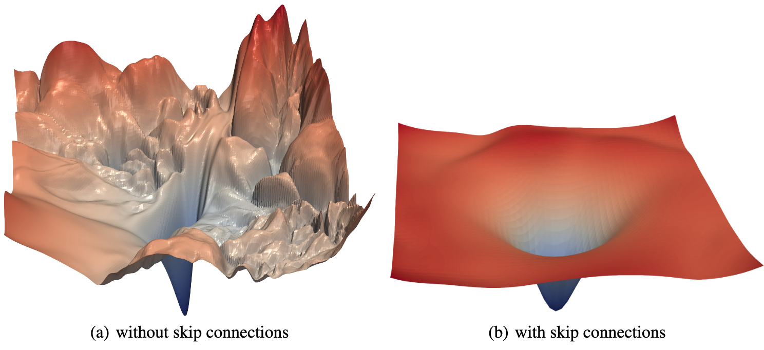
此外, 由于需要进行残差连接, 因此需要注意数据的维度, 从而使得 $\mathbf{x}$ 和 $\mathbf{g}(\mathbf{x})$ 的维度一致, 从而可加. 例如下图, $1\times 1$ 卷积层的作用就是将输入的维度进行调整, 使得其与输出的维度一致.

完整的 ResNet-18 结构如下:

ResNet 的实现和 GoogLeNet 类似, 但其参数更少, 架构更简洁, 也因此更受欢迎.

Related Notes

• Convolutional Neural Networks
• CNN Architecture